#What's my problem?

I want to have some abstract little numbers next to the rules of a formal grammar, which will be transformed according to some abstract rules (not necessarily multiplication or addition) to achieve certain goals.

#What goals?

I'm writing a parser that will approximate natural language with context-free grammars. Obviously, since this is an approximation, nothing can be absolutely correct and exact. So some rules may approximate certain phrases better and others worse. For that I need little numbers that get transformed somehow, so that the output looks roughly like this: for this phrase, such-and-such a fact is 57% likely to be correct, and for that phrase, 98% likely to be correct.

#Why are the numbers abstract, what do you want from them?

I wanted a convenient interface for specifying these numbers, one that can be interpreted logically and that is easy to write as a user of the parser (that is, without getting into numerical methods).

#Well, there are ordinary probabilities, for example: numbers from 0 to 1, just take them and multiply.

No. Ordinary probabilities don't fit, for several reasons:

• The longer the phrase, the more multiplications of numbers from 0 to 1, and the closer the result gets to 0.
• Because of this, the absolute values of the "probabilities" make no sense at all.
• They're inconvenient to specify: you need some magic numbers like 0.57, 0.98, 0.05.
• They come with the constraint that the probabilities for one nonterminal must sum to 1.
• See the example in /199 (in Russian)

I think that clears things up, so now I'll continue with the regular story.

In /184 (in Russian) I proposed an interface for describing "abstract numbers" that can be interpreted logically:

• +20% means that something increases by something, and it increases by more than +10% would
• -20% is the same as above, but it decreases, and decreases more strongly than -10%
• 60% sets an ordinary probability

Soon I realized that you can't mix ordinary probability with these +20%, -20%. Because the ordinary probability eats them up and generally infects everything with itself.

So we throw it out and add an element: 0%, which means that nothing changes.

Let's call this quantity "confidence". And let's introduce an operation for combining "confidences", denoted by the symbol ★.

Now the main problem is to define how these confidences are specified, what properties they have and how to compute ★.

I decided that -20% should map to -0.2, +20% to +0.2, and in the end the domain should be [-1; 1].

I started by creating this function.

×1.2
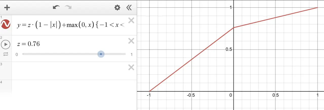
png

Its problem is that it isn't smooth, and it gives different results depending on the order in which you apply it. And in grammars there is no fixed order, and you don't know when ★ should be applied and when not. On top of that, it took inputs in [-1; 1] but returned values in [0; 1]. But that's easy to fix.

So the most important property I need is: (a ★ b) ★ c = (a ★ c) ★ b.

Next I tried googling, to no avail. I tried reading about Bayes' theorem and thinking about how to apply it to my problem, also to no avail.

Then I realized that I could use brute force!!! I'm a damn numerical methods programmer, I should use that to find the function I need numerically!

So I had to do the following sequence of steps:

• Formulate the properties of the function I need
• Program the computation of how well these properties hold, using integrals
• Find a library for defining smooth 2D functions by a set of numbers
• Use optimization methods to find the numbers that give the minimum of these integrals
• Optimize well enough and use it

I thought that such a function might not exist; it had to be just too good.

I formulated the properties easily, wrote the integral and started testing. My linear function scored 2 on these properties, while the ideal function should score 0. The worst part was the triple integral for the most important property (so an accuracy of 10 points per dimension took 1000 function evaluations).

I didn't find a library for building smooth 2D functions, so I had to apply my knowledge of FEM and program the evaluation of the function from point values myself.

For the optimization methods (finding the minimum of a function) I took argmin-rs. I recommend quasi-Newton methods.

Then I combined all of this with the optimization methods and...

It ran for a very long time. To define the 2D function I required too many parameters, and many of them were redundant, so a ton of time was wasted.

Then I realized that I needed visualization! And right at that moment Anton (in Russian) wrote about embedding Python in Rust! After a bit of a fight with it, I managed to plot the resulting function with matplotlib, and even plt.show() worked!

I plotted the graph, and...

×1
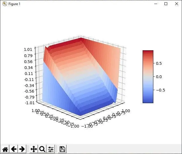
jpg

The function turned out... awful: it was very noisy, non-monotonic, and clearly overfitting somewhere. And the metric barely crawled down to 0.04. I left the optimization running for several hours, to no avail: in the end I got complete nonsense, and degenerate nonsense at that, a function that tends to just keep the first value.

I was really upset.

But the next day it occurred to me that my "weights" from /199 (in Russian) were actually a very good fit! They were perfect for the interval from 0 to 1 and for multiplying 0.8 by 1.2, but were inconvenient for the interval from 1 to ∞. So I decided to simply fold this infinity down to 1 by division. Then +20% turned into 1+1/(1-0.2)=2.25. And you know what? I got the perfect function I wanted! It satisfied all the properties perfectly and was really smooth. And it's also symmetric: from -1 to 0 it behaves the same way as from 0 to 1.

Ah, so simple. And I didn't even believe it existed.

×1
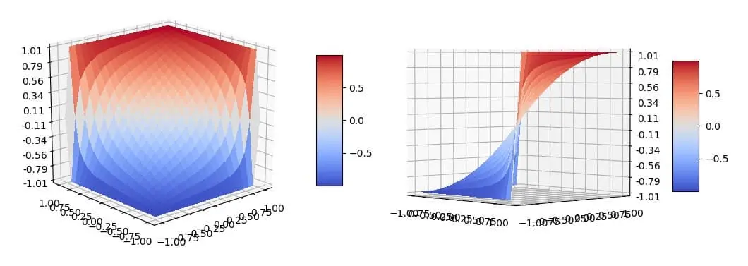
jpg

Here it is, my perfect function ❤️

And you can play with it here.

I published the result here: github:confidence (in Russian); I tried to write the code very cleanly and safely. In the end I realized that float is dynamic typing at the processor level, and I want it to be built on algebraic data types :)))

But that's a whole different story, and the topic of the next post...

#The interval [-1, 1]

In general, I really love the interval [-1, 1].

A year ago, when I was writing my term paper (in Russian) on FEM, I had to study how well the method works on non-uniform square grids and produce plots or tables.

If you don't know what a non-uniform grid is, here's an illustration (which I drew with code). The property of this grid is that each next element is c times larger than the previous one, where c is some positive number from 0 to ∞.

×1
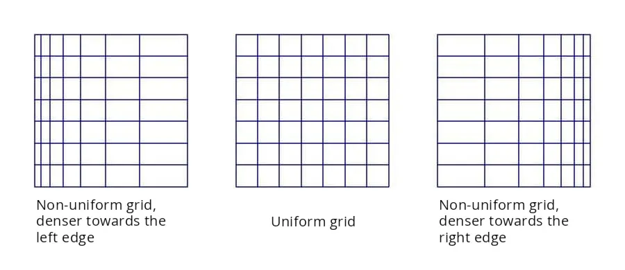
jpg

Everyone usually made tables: they took a few non-uniform grids and the accuracy on each, and drew some conclusions. But I'm a goddamn perfectionist: I made the computer work its transistors to the bone, so I swept through everything I could with a very small step and plotted graphs in LaTeX.

At first, like everyone else, I set the number c from 0 to ∞. So the closer c is to zero, the denser the grid gets towards the right edge, and the closer it is to infinity, the denser towards the left.

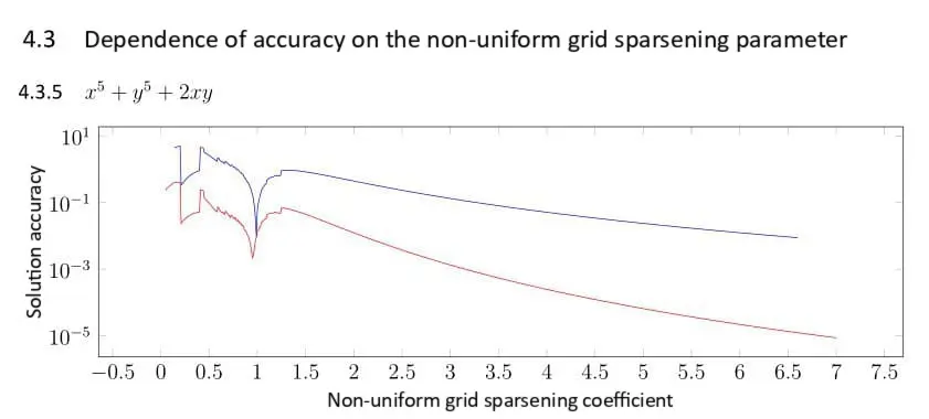
But doing research on something that goes to infinity is inconvenient; look at this graph:

×1
jpg

Where do I stop here? At 10^5? At 10^10? Make x grow exponentially and use a logarithmic scale? Who knows. Besides, it's very inconvenient to reason about logically: left and right somehow end up asymmetric.

So I decided to come up with a function that makes specifying non-uniform grids very convenient: with a coefficient of -1 the grid gets denser towards the left edge, and with a coefficient of 1 it gets denser towards the right edge.

4.2.2 Non-uniform grid functions

While doing the lab work, I found a function that makes it easy to specify a non-uniform grid that gets denser towards one of the ends.

If the grid starts at $a$ and ends at $b$, and the number of elements is $n$, then the grid can be defined as follows:

$$x_i = a + m\left(\frac{i}{n}\right)\cdot(b-a),\quad i=\overline{0,n}$$

where $m(x)$ is some function that defines the non-uniform grid. Here $x$ must belong to the interval $[0, 1]$, and the function $m$ must return values from the same interval and be monotonic on it. Then the grid is guaranteed to be monotonic, that is, $j \leqslant i \Rightarrow x_j \leqslant x_i$.

Example: with $m(x) = x$ the grid becomes uniform.

The function I found depends on the non-uniformity parameter $t$:

$$m_t(x) = \frac{1-(1-|t|)^{x \operatorname{sign} t}}{1-(1-|t|)^{\operatorname{sign} t}}$$

This function degenerates into $x$ at $t = 0$; at $t = -1$ it degenerates into a grid that lies entirely at 0; and at $t = 1$ it is entirely concentrated at 1.

Thus, you can study various non-uniform grids by changing the parameter from $-1$ to $1$, where the point $t = 0$ gives the result on a uniform grid.

I came up with it and described it (in Russian) in the report.

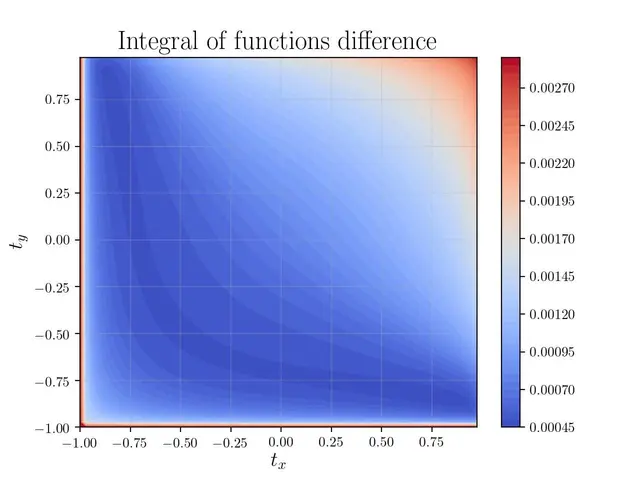
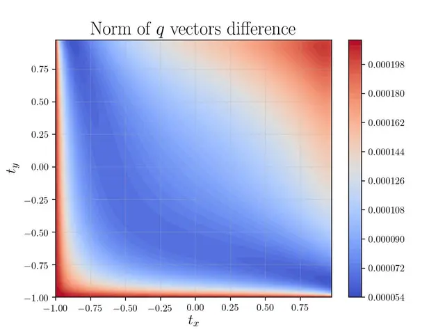
And this is how awesome the studies look when the grid parameter is varied along both the X and Y axes at the same time.

×2
jpg

×2
jpg

#Update from 21.12.2024

A new AI model, o1, came out recently, and I asked it to design a function that would handle these probabilities, and it made a very neat and compact alternative function that meets my requirements. Below are my prompt and its solution. When I was writing this article, I couldn't even imagine that some automated system would be able to help me with this problem. Truly, we have entered a new era of technology.

You can look at this function in Desmos: https://www.desmos.com/calculator/gzejyiee3u

# Confidence function

Suppose we're writing a parser that assigns a probability to each grammar rule. If a rule has been parsed, we multiply the total by its probability.

In this case, the problem with classical probabilities, numbers from 0 to 1, is that for a large amount of parsed text the total probability will be very small. And it's hard for us to judge how confident we are in that result.

This repository presents the `confidence` data type, whose multiplication makes it possible to represent such confidence. This data type has three different states:
* The degree of confidence that the hypothesis is false
* Complete uncertainty
* The degree of confidence that the hypothesis is true

Its domain is `A = [-1, 1]`:
* The range `[-1, 0)` represents confidence that it is wrong. The closer to `-1`, the greater this confidence
* The element `0` means that it is unknown whether it is right or not
* The range `(0, 1]` represents confidence that it is right. The closer to `1`, the greater this confidence

The multiplication method is overloaded for these "confidences". Let's denote it as `P(a: A, b: A) -> A`, that is, the function takes two arguments from the domain `A` and returns a result from the same domain. This function has the following properties:
* `P(x, 0) = x`
* `P(x, -1) = -1`
* `P(x, 1) = 1`
* `P(x, +y) >= x` - positive values increase it
* `P(x, -y) <= x` - negative values decrease it
* `P(P(x, y), z) = P(P(x, z), y)` - the result is the same regardless of the order of application. This is very important, because during parsing there can be many options for the order in which to apply the function, and a lot depends on it.
* `P(x, y)` is monotonically increasing in `y`.
* `P(x, y) = P(y, x)` - this property wasn't needed for parsing, but it appeared by accident